Setting the supplier and consumer risk. How amendments to the trade law affected retail and customers. Market at a fork - in the face of deferred risks

When accepting a batch of products, control may be solid, when each unit of product is controlled (for example, a bearing, a bottle of water, a coil of wire, etc.). Such control is most often economically unjustified and sometimes impossible. More common selective control, when a conclusion about the quality of a batch of products is made based on an analysis of a limited sample. Selective control is divided into:

by time: input (purchase control of raw materials and semi-finished products), intermediate (interoperational) and output (acceptance and certification of finished products);

according to changes as a result of control: destructive and non-destructive (for example, to control the strength of a product it must be brought to destruction);

by hardness: normal, reinforced (more complex) and lightweight; the transition from one type of control to another is made depending on the number of batches that were sequentially accepted, or, conversely, rejected by the consumer;

according to the controlled parameter: quantitative (in this case, the controlled indicator of product quality is measured) and qualitative (in particular, the most common control is based on an alternative criterion, when a conclusion is made about each controlled object, whether it is suitable or unsuitable, meets the requirements or does not meet) .

Control plan- this is a system of rules for selecting products for inspection (forming samples) and making a decision regarding the entire batch - to accept the batch or reject it. The rejected batch is either returned to the supplier or is subject to complete inspection. The application of a statistical control plan is essentially a test of the statistical hypothesis H 0:. the quality of the batch meets the requirements under the alternative hypothesis H 1: the quality of the batch does not meet the requirements.

The most common control is based on an alternative criterion. Suppose that in a batch of N products there are M defective products (M is unknown). It is required to estimate the general share of defective products q = M/N.

based on the results of monitoring a sample of n products, of which m are defective.

The following types of control plans are distinguished:

single stage: if among n products the number of defective t does not exceed the acceptance number c (t< с), то партия принимается, в противном случае партия бракуется;

two-stage: at the first stage, if among n 1 products in the sample the number of defective t 1 does not exceed the acceptance number c 1 (m< с 1), то партия принимается; если т 1 >d 1, where d 1 is the rejection number, then the batch is rejected; if from 1< m 1 < d 1 , то принимается решение о взятии второй выборки; на второй сту­пени объемом п 2 с приемочным числом с 2 , если суммарное число дефектных изделий не превышает с 2 (m 1 + т 2) < с 2 , то партия принимается, в противном случае партия бракуется;

multi-stage plans- generalization of a two-stage plan. A sample of volume n 1 is taken and the number of defective products t 1 is determined; at m 1< с 1 , партия принимается, при с 1 < m 1 < d 1 (d 1 >with 1 + 1), a decision is made to take a second sample of size n 2. Let among (n 1 + n 2) products there are (m 1 + m 2) defective, then if (m 1 + m 2)< с 2 (с 2 - приемочное число второй ступени), то партия принимается, при с 2 < (m 1 + т 2) < d 2 (d 2 >with 2 +1), a decision is made to take the third sample, etc. At the final k-th step, if among the sum (n 1 + n 2 + + ... + n k) of inspected products there were (t ( + t 2 + + ... + t k) defective and (t 1 + t 2 + ... + t k) with k, then the batch is accepted, otherwise the batch is rejected. In multi-stage plans, the number of steps k is specified in advance. Usually n 1 = n 2 = ... = n k.;

sequential control, in which the decision is made after evaluating a number of samples, the total number of which is not established in advance, but is determined in the control process based on the results of previous samples. One of three decisions is made - accept the batch, reject the batch, continue control.

Operational characteristics of the plan

The decision on the quality of the entire batch of products is made based on sample observations. There are two types of risks:

There were a large number of defective products in the sample, but their share in the entire batch was acceptable (the batch was good, but the sample was bad). In this case, a valid batch will be mistakenly rejected - this is an error of the first type. The probability of such an error α – supplier risk. The probability of acceptance of the batch in this case is equal to (1 – α);

if the batch is heavily contaminated with defective products, the sample may contain a small number of defects (the batch is bad, but the sample is good) and the batch will be mistakenly accepted - an error of the second type. The probability of such an error is β – consumer risk.

It is required to give a conclusion about the quality of a batch of products based on the proportion of defects q (group indicator of product quality). Let us assume that the normative value of this indicator q 0 is given, denoted in the NQL standards: NQL = q 0 (Normative Quality Level). The normative level of nonconformities NQL is the boundary value of the level of nonconformities: a batch of products is considered fit for delivery and for intended use by the consumer if the actual level of nonconformities does not exceed the normative value NQL.

Then the task is to test the hypothesis that the proportion of defective products q in the batch is equal to the permissible value q 0, i.e. Н 0: q = q 0 and at the same time make the risks of the supplier and consumer unlikely.

The main probabilistic indicator of the statistical control plan is the operational characteristic. This is a function P(q), which determines the probability of acceptance of a batch of products depending on the proportion of defective products q = M / N. Obviously, each plan will have its own operational characteristics.

Let it be established that if q< q 0 , то качество партии счи­тается хорошим и партию следует принять. При q >q 0 lot should be rejected. Ideally, the operational characteristic will be the function P(q) = 1 at 0< q < q 0 , P{q) = 0 при q 0 < q < 1 (рис. 5.2). Такая характеристика соответствует плану сплошного контроля при условии, что во время контроля дефект не может быть пропущен.

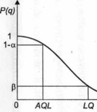
With selective control, the operational characteristic is a smooth curve (see figure), with P(0) = 1, i.e. a batch in which all products are suitable cannot be rejected; P(1) = 0: a batch in which all products are defective cannot be accepted.

P(q)

Usually, batches are divided into “good” and “bad” using two numbers: q 0 = AQL (Acceptable Quality Level) - acceptable quality level, q 1 = LQ (Limiting Quality) - limiting quality.

Acceptable quality level AQL is the maximum level of nonconformities in a batch of products that is considered satisfactory upon acceptance (according to outdated but practically used terminology, the acceptance level of defects). When inspected based on this indicator, the majority of submitted lots will be accepted if their level of non-conformity does not exceed the specified AQL value.

Limit quality LQ (in outdated terminology – defectiveness level) is the minimum level of non-conformities that is considered unsatisfactory upon acceptance. Inspection based on the LQ indicator ensures a low probability of acceptance of an individual batch.

The games are considered good for q< AQL и плохими при q >LQ. At AQL< q < LQ качество партии считается еще допустимым.

The plan has requirements: the probability of acceptance for a good batch must be no lower than 1 – α, for a bad batch – no higher than the consumer’s risk β (see figure):

P(q) >1– α at q< AQL;

P(q)< β при q >L.Q.

those. The plan boils down to ensuring that the risks of the supplier and consumer do not exceed aiβ.

With α = 0.05, β = 0.1, AQL = 0.003, LQ = 0.02 - for this plan, on average, out of every 100 batches with contamination no higher than 0.3%, no more than five will be rejected, and out of 100 batches containing more than 2% defective products will be accepted no more than 10 batches.

Control by alternative criteria is a control in which a conclusion is made about each controlled object whether it is suitable or not suitable, meets the requirements or does not comply.

Let's assume that a batch of N products is being inspected. For control, a random sample of n is made. The number of ways in which n products can be selected from N without taking into account the order of occurrence is the number of combinations

Let the random variable X be the number of defective (non-conforming) products in the sample. It is known that in the entire batch of products the proportion of nonconformities is q. Then the number of defective products in the batch is equal to Nq, the number of suitable products will be N – Nq. Consider the event X = t - exactly t defective products were taken. This is possible if t products are taken from Nq defective products, and n - t products are taken from the remaining good ones N – Nq (there are n products in total in the sample). Then the probability of the event in question

(5.1)

Formula (5.1) describes the hypergeometric distribution.

As a rule, the sample size is no more than 10% of the entire batch, in which case the hypergeometric distribution can be approximated by the binomial

P(X = m) =C m n q m (1-q) n-m . (5.1)

In practice, the proportion of mismatches is usually less than 10%, in which case the binomial distribution can in turn be approximated by the Poisson distribution:

(5.3)

Let's consider single-stage control based on an alternative criterion. The probability of acceptance of the batch P(q) in this case is the probability that the number of defective products t in the sample will not exceed the acceptance number c. Using the formula for adding the probabilities of incompatible events, we obtain the equation for the operational characteristics of a one-stage control plan:

P(q) = P(t< с) – Р(Х = 0) + Р(Х = 1)+...+ Р(Х = с) =

Substituting into the resulting expression instead of P(q) the formula of the corresponding distribution (binomial or hypergeometric or Poisson distribution), we obtain the equation for the operational characteristics of a single-stage plan. Substituting the known values ​​of AQL and LQ, as well as the given risks α and β, we obtain a system of nonlinear equations, solving which we find the plan parameters - sample size n and acceptance number c.

Analysis of the corresponding dependencies shows that with a constant sample size n, with an increase in the acceptance number c, the probability of accepting a batch with a given acceptable quality level AQL increases (Fig. 5.4, a), and with an increase in n at a constant c, the probability of accepting a batch decreases (Fig. 5.4, a). b). It is possible to select a control plan (p,c) that would provide risk values ​​air for given values ​​of quality levels AQL and LQ.

Rice. 5.4. Operational characteristics for n = const (a) and c = const (b)

Based on the results of the inspection of many batches of products, some useful characteristics can be found, in particular, the average proportion of nonconforming units of product in accepted batches (average level of output quality) and the average number of items inspected in the batch.

Let's consider a one-stage plan, in which rejected batches of products are subject to continuous control, i.e. All remaining (N-n) products of the batch are controlled, and identified defective products are replaced with suitable ones. Let us assume that the proportion of defective products is constant and equal to q. Then, with probability P(q), batches of products are accepted (the proportion of defective products in it is approximately equal to q), and with probability the batches are subject to continuous inspection; the proportion of defective products in these batches is zero. Then the average proportion of defective products in accepted batches according to the mathematical expectation formula for a discrete random variable is equal to:

q cp =qP(q) + 0 = qP(q). (5.7)

The value q cp is called the average level of output quality. From formula (5.7) it is clear that at q = 0 the value of q c = 0 and at q = 1 also q cp - 0, since the probability P(1) = 0. Since q cp is a non-negative function of q, equal to zero at q = 0 and q = 1, then within the interval 0< q < 1 средний выходной уровень дефектности имеет максимум q max (рис. 5.5). Максимальный для заданного плана контроля средний уровень q max называют пределом среднего уровня выходного качества.

P When using the plan discussed above, when rejected batches of products are subject to continuous inspection, the number of products inspected in a batch of volume N is a random variable that takes the value n with probability P(q) and the value N (continuous inspection) with probability . Therefore, the average number of inspected products in a batch is equal to:

n cp = nP(q) + N(1 -P(q)). (5.8)

If a decision is made to return the rejected batch to the supplier, then the scope of control in this case is constant and equal to the sample volume n.

To reduce the amount of control, multi-stage and, in particular, two-stage plans are used. Two-step control reduces supplier risk.

With sequential control, products selected from a batch are checked at random, and at each step one of three decisions is made: accept the batch, reject the batch, or continue control - take control of the next product. Control continues until sufficient information is accumulated to make a decision.

In sequential control based on an alternative criterion, the risks of the supplier α and the consumer P, the acceptable level of quality AQL = q 0 and the maximum quality LQ = q v are taken as the initial data. After setting these parameters, hypotheses H 0 are tested: q< q 0 или H 1: q>q 1 Sequential analysis methods are used that have already been used to derive basic relationships for control charts of cumulative sums. The probability P(q 0 ,n) is determined that “the inspected products belong to a batch with a share of nonconformities not exceeding q 0 ; or the probability P(q l ,n) that they belong to a party with a share of nonconformities no lower than q v . To make a decision, find the likelihood ratio P(q 1 ,n) / P(q 0 ,n).

Statistical control plans and decision rules. A statistical control plan is understood as an algorithm, i.e. rules of action, the input is the general population (product batch), and the output is one of two decisions: “accept the batch” or “reject the batch.” Let's look at a few examples.

Single-stage control plans: select a volume sample; if the number of defective units in the sample does not exceed , then accept the batch, otherwise reject it. The number is called acceptance.

Special cases: plan - accept a batch if and only if all units in the sample are suitable; plan - the batch is accepted if all units in the sample are suitable or exactly one is defective, in all other cases the batch is rejected.

Two-stage control plan : select the first volume sample; if the number of defective units in the first sample does not exceed , then accept the batch; if the number of defective units in the first sample is greater than or equal to , then reject the batch; in all other cases, i.e. when more but less, a second volume sample should be taken; if the number of defective units in the second sample does not exceed , then accept the batch, otherwise reject it.

Let's take a plan as an example. First, the first sample of volume 20 is taken. If all the units in it are suitable, then the batch is accepted. If two or more are defective, the lot is rejected. What if only one is defective? In a real situation, in such cases, disputes begin between representatives of the enterprise and environmental control, or the supplier and the consumer. They say, for example, that a defective unit accidentally got into the lot, that competitors slipped it in, or that during inspection an incorrect conclusion was accidentally drawn. Therefore, in order to stop disputes, they take a second sample of volume 40 (twice as large as the first time). If all units in the second sample are suitable, then the batch is accepted, otherwise it is rejected.

In actual regulatory and technical documentation - supply contracts, standards, technical specifications, instructions for environmental control, etc. - statistical control plans and rules are not always clearly formulated decision making. For example, when describing a two-stage inspection plan, instead of specifying the acceptance number c, there may be a mysterious phrase “the inspection result of the second sample is considered final.” It remains to be seen how to make a decision on the second sample. A manager, administrator (civil servant), ecologist or economist involved in environmental or quality control issues should first strive to achieve crystal clarity in the formulation of rules decision making, otherwise erroneous and unfounded decisions, and therefore losses, are inevitable.

Operational characteristics of the statistical control plan. What are the properties of a statistical control plan? They are usually determined using a function that connects the probability of defectiveness of a control unit with the probability of a positive assessment of the environmental situation (batch acceptance) based on the control results. In this case, the probability that a particular unit is defective is called the input defect level, and the specified function is called the operational characteristic of the control plan. If there are no defective units, then the batch is always accepted, i.e. . If all units are defective, then the batch is likely to be rejected. Between these extreme values ​​the function decreases monotonically.

Let's calculate the operational characteristics of the plan. Since the batch is accepted if and only if all units are suitable, and the probability that a particular unit is suitable is equal to , then the operational characteristic has the form

Operational characteristics for specific statistical control plans do not always have such a simple form as in the case of formulas (5) and (6). Let's take a plan as an example. First, let's find the probability that the batch will be accepted based on the results of the control of the first batch. According to formula (5) we have:

The probability that control of the second sample will be needed is equal to

In this case, the probability that, based on the results of its control, the batch will be accepted is equal to

Therefore, the probability that the game will be accepted on the second attempt, i.e. that when testing the first sample, exactly one defective unit will be detected, and then when testing the second, none is equal to

Therefore, the probability of accepting the game on the first or second attempt is equal to

In the practical application of statistical acceptance control methods, to find the operational characteristics of control plans, instead of formulas that have a visible appearance only for certain types of plans, numerical computer algorithms or pre-compiled tables are used.

Supplier risk and consumer risk, acceptance and rejection defect levels. Important concepts associated with operational characteristics acceptance and rejection levels of defects, as well as the concepts of “supplier risk” and “consumer risk”. To introduce these concepts, two characteristic points are identified on the operational characteristic, dividing the input defect levels into three zones - A, B and C. In zone A, everything is almost always good, namely, the environmental situation is almost always considered favorable, almost all parties are accepted. In zone B, on the contrary, everything is almost always bad, namely, environmental control almost always detects environmental violations, almost all batches are rejected. Zone. B - buffer, transitional, intermediate, in which both the probability of acceptance and the probability of rejection differ markedly from 0 and 1. To set the boundaries between zones, two small numbers are chosen - the risk of the supplier (manufacturer, enterprise) and the risk of the consumer (customer, environmental system control), while the boundaries between zones set two levels of defects - acceptance and rejection, determined from the equations

Thus, if the input defectiveness level does not exceed , then the probability of batch rejection is small, i.e. does not exceed . The acceptance level of defects identifies a zone of values ​​of the input level of defects, in which violations of environmental safety are almost always not noted, batches are almost always accepted, i.e. the interests of the inspected enterprise (in the environment) and the supplier (in quality control) are respected. This is the supplier's comfort zone. If it provides operation (defect level) in this zone, then no one will disturb it.

If the input defectiveness level is greater than the defectiveness rejection level, then violations are almost certainly recorded, the batch is almost always rejected, i.e. environmentalists learn about violations, the consumer is protected from receiving shipments with such a high level of defects. Therefore, we can say that the interests of consumers are respected in the zone - defects do not fall to them.

When choosing an inspection plan, they often start by choosing acceptance and rejection defect levels. In this case, the choice of a specific value for the acceptance level of defects reflects the interests of the supplier, and the choice of a specific value for the rejection level of defects reflects the interests of the consumer. It can be proven that for any positive numbers and , and any input defectiveness levels and , and less than , there is a control plan such that its operational characteristic satisfies the inequalities

In practical calculations, (i.e. 5%) and (i.e. 10%) are usually taken.

Let's calculate the acceptance and rejection defect levels for the plan. From formulas (5) and (7) it follows that

Since the supplier’s risk is small, then from the known relation of mathematical analysis

the approximate formula follows

For the defectiveness rejection level we have

In the practical application of statistical acceptance control methods to find acceptance and rejection levels of defects in inspection plans, instead of formulas that have a visible appearance only for certain types of plans, numerical computer algorithms or pre-compiled tables available in regulatory and technical documentation or scientific and technical publications are used.

Limit of average output defectiveness level. Let's discuss the fate of the rejected batch of products. Depending on the situation, this fate may be different. The batch can be disposed of. For example, a rejected batch of nails may be sent for melting. The lot may be downgraded and sold at a lower price (in this case, the results of sampling will not be used to verify that a given quality level is being met, but to assess the actual level of quality). Finally, a batch of products can be subjected to complete control (for this, engineers from all plant services are usually involved). During continuous inspection, all defective products are detected and either corrected on site or removed from the batch. As a result, only suitable products remain in the batch. This procedure is called "

Techniques for reducing risks associated with sampling

Sampling inspection always involves risks of both accepting low quality products and rejecting high quality products, but these risks should be acceptable provided that the AQL and inspection level are chosen correctly.

If a supplier or customer feels that their risk is too high in a particular case, the appropriate AQL and control level can be checked. It is assumed that they are assigned correctly.

The manufacturer is interested in reducing risk in cases where the quality is better than the AQL (he cannot reduce risk in any other way). The consumer will be especially interested in the risks in cases where the quality is worse, since if the quality is better than the AQL, he receives the required quality.

Three methods can be used to reduce risks for each party.

The first method is to improve production. It may seem that this path is obvious, but when discussing sampling plans, OX curves, switching rules, etc. You can forget about the elementary rule according to which, with a low percentage of non-conforming units, the consumer certainly receives what he needs, and a high probability of acceptance is achieved for the manufacturer.

The second method is applicable only in the special case with an acceptance number equal to 0. Plans with a zero acceptance number have such flat OX curves that large risks are inevitable.

For this reason, GOST R 50779.71 allows the use of an alternative method in cases where the tables lead to a zero acceptance number (with the approval of the authorized body). In this case, plans are used for the same AQL, but with an acceptance number of 1 instead of 0. Approximately four times the sample size required for an acceptance number of zero would be required. But the risks on both sides are greatly reduced, which often justifies these costs.

Costs can be somewhat reduced by using two-stage and multi-stage control. These alternatives are available when the acceptance number is 1 or more. Sequential monitoring is possible but is not the subject of this standard.

The third method considers the possibility of increasing the batch size. If the lot size is increased enough to change the code and increase the sample size, this will reduce the risk of the parties, since the larger sample size corresponds to a more curved curve, and the tables are designed so that this curve will be higher than the previous curve for most points with quality better than AQL and lower at most points where quality is worse than AQL. It is not possible to construct tables preserving these properties without losing other necessary properties. Figure 28 shows that, for example, four normal control plans correspond to AQL = 1.5%. For better quality AQL, it can be seen that the larger the sample, the higher the proportion of accepted lots, while for worse quality AQL, with the maximum sample, the most lots are rejected, and with the minimum sample, the least is rejected (it is desirable that the plan rejects lots as often as possible, when the quality is worse than AQL).

Figure 28 - Four one-stage sampling plans for AQL = 1.5% nonconforming units under normal inspection

Increasing lot sizes to provide better inspection protection may be discussed as it is not always easy or reasonable to change the lot size. It must be linked to the duration of the technological process, the volume of products that can be processed simultaneously, transport difficulties, warehousing problems, etc. In all other circumstances, increasing the batch size may be beneficial from the manufacturer's point of view.

When studying the height of the curves in Figure 28 at points two, three, four times larger than AQL, it should be remembered that the curves show only a section of the picture (the normal control section). For almost all normal control plans according to GOST R 50779.71, the expected percentage of accepted lots with quality twice as bad as AQL is less than 80%. This acceptance rate will always lead to increased control.

This technique is not always justified, but the parties can discuss the choice of plan directly on the basis of the OX curves.

13.Sampling plans. Single-stage, two-stage, multi-stage plan. Types and levels of control. Rules for switching between different types of sampling control.

The tables of GOST R 50779.71-99 propose three types of sampling plans - one, - two and multi-stage plans. If you have multiple plan types for a given AQL and sample size code, you can use any of them. The decision to select a plan type is based on a comparison of organizational issues and sample sizes. Sample size codes are given in Table 1 of the standard and presented in Appendix 5.

Single-stage sampling plan.

The number of controlled products must correspond to the sample size of a one-stage plan. The sample is selected randomly after all units have been formed into a batch, or during its production time. After selecting the sample, the quality parameters of each product included in the sample are monitored, the measurement results are entered into a control sheet, the form of which is shown in Fig. 14, and the number of non-conforming units is counted. If the number of nonconforming units in the sample is equal to or greater than the rejection number, the lot is considered unacceptable. With weakened control, the sample may contain the number of nonconforming units of product between the acceptance and rejection numbers. Under these conditions, the lot is determined to be acceptable, but normal inspection is resumed starting with the next lot. The scheme of single-stage sampling control is shown in Fig. 15.

Two-stage sampling plan

The number of controlled units should correspond to the sample size of the first stage of this plan. If the number of nonconforming units in the first sample is equal to or less than the first stage acceptance number, the lot is considered acceptable. If the number of nonconforming units found in the first sample is equal to or greater than the first stage rejection number, the lot is considered unacceptable.

If the number of non-conforming units of the first sample lies in the range of the acceptance and rejection numbers of the first stage, it is necessary to control the second sample. The number of non-conforming units found in the first and second samples is summed. If the cumulative (total) number of nonconforming items is equal to or less than the second stage acceptance number, the lot is considered acceptable. If the cumulative number of nonconforming items is equal to or greater than the second stage rejection number, the lot is considered acceptable. The scheme for carrying out two-stage sampling control is shown in Fig. 16.

When using a multi-stage sampling plan, the standard provides for the ability to extract up to seven samples. After extracting the first sample, product quality indicators are monitored, the number of non-conforming products is calculated and compared with the acceptance and rejection numbers of the first stage. If the number of non-conforming products:

Does not exceed the acceptance number of the first stage Ac 1 – the batch is accepted;

Exceeds the first stage rejection number Re 1 – the batch is rejected;

Located between the acceptance and rejection numbers - a second sample is made.

After monitoring quality indicators, the total number of non-conforming products from both samples is calculated and compared with the acceptance and rejection numbers of the second stage. If the total number of nonconforming products.

Assessments of supplier quality systems and acceptance control.

Relationship between the scope of control and the value of consumer risk.

Total risk for the consumer.

The concept of “customer risk under supplier control” introduced in this standard is of a conditional nature. The corresponding value characterizes the maximum probability of making a positive decision based on the control results, provided that the quality of the population, for example a batch of products, does not meet the established requirements. At the same time, the probability of delivering a batch of inappropriate quality can be very different. For a supplier with a reliable reputation, having certificates from reputable organizations for quality systems, this probability is low. On the contrary, for a supplier who does not have such certificates, does not know quality management methods, and is unable to ensure the stability of production processes, there is a high probability of delivering a batch of inappropriate quality.

The consumer is interested in the total risk, which takes into account both the probability of a set of products being submitted for control of inappropriate quality and the probability of the control procedure missing such products. In the literature on mathematical statistics, such a risk is usually called Bayesian. It is calculated taking into account a priori information, ᴛ.ᴇ. information available prior to quality control.

Protecting the consumer by reducing the standard value of the conditional risk b 0 is an expensive means. Figure 3 and Table 1 show the dependences of the control volumes n on the risk b 0 . They show how quickly the volume of control grows, and therefore the cost of control, as b 0 decreases.

In cases where the a priori probability of receiving batches of products of inadequate quality is small, for example less than 10 -1 ... 10 -2, it is not extremely important to set a small value of b 0. This only leads to an increase in the cost of control.

The system established by this standard protects the consumer not by establishing small values ​​of b 0, but by giving the consumer the right to set b 0 independently on an individual basis (without coordination with anyone).

If the consumer is not confident in the reliability of information about the quality of the supplied products, then he can protect himself by reducing b 0, which leads to an increase in the cost of production.

The relationship established by this standard encourages both parties to focus on quality assurance systems and their assessments rather than on quality control. The better the supplier’s quality assurance system works and the more information the consumer has about it, the cheaper the acceptance control.

This standard provides the consumer with the opportunity to waive acceptance inspection or accept part of the lot without inspection, using lower-cost means of protecting themselves from the delivery of poor quality products, such as inspections of supplier quality systems and analysis of inspection and test data obtained during production.

Figure 3 - Dependence of sample volumes for one-stage (upper curve n 1) and two-stage (lower curve n 2) control on the consumer risk when monitoring the supplier b 0 for batch size N.

SPC plans are characterized by consumer, supplier risks or corresponding levels of confidence.
The risks of the consumer and supplier are characteristics of the reliability of decisions made based on the results of the SPC (hereinafter referred to as the reliability of the SPC). These characteristics determine the probabilities of correct (correct) and erroneous decisions made based on the results of the SPC.
SPC schemes are characterized by scheme-average consumer risks or scheme-average supplier risks.
The choice of specific plans and (or) SPC schemes is carried out by the party organizing control, without agreement with anyone, and it must ensure the specified reliability of decisions affecting the interests of the other party, namely:
- when monitoring the supplier, the specified (standard) value of the consumer’s risk must be ensured;
- when monitoring the consumer, the specified (normative) value of the supplier’s risk must be ensured.
Consumers have the right to change the standard values ​​of risks and average consumer risks under the control of the supplier or the corresponding levels of confidence in the ranges specified in this standard, depending on the degree of their confidence in the supplier’s information about product quality. With a high degree of trust, they can increase risks up to values ​​that mean a transition to acceptance of products without control by the supplier.
In the case of product release without a contract, the standard value of the consumer's risk during supplier control is established by the body that issued the certificate for the product or quality system. This body may change the value established by it based on the results of product supervision.
When releasing products without a contract, the supplier, who does not have a certificate for the product or quality system, establishes the degree of trust (the standard value of the consumer's risk during supplier control) independently, unless otherwise established by law or government regulations, indicating this value in the quality system documents, as well as documents accompanying the products.
In the case of a SPC during arbitration or judicial consideration of a dispute between a manufacturer (supplier) and a consumer, the choice of control plan and scheme is carried out by the party applying to arbitration or court, while the other party must be protected from possible erroneous decisions by establishing restrictions on the values ​​of the corresponding risks or levels trust.
When conducting SPC by a third party, by court decision in cases determining the responsibility of the supplier (manufacturer) for the release of products that do not meet the requirements of the standards or the supply agreement, restrictions on the supplier’s risk must be met.
In the case where the final control and acceptance by the manufacturer are carried out using continuous statistical acceptance control (products are received for control piece by piece using the “flow” method), the consumer or the inspecting authorities can, when checking the correctness of the final control and acceptance, form products into batches of any size. Claims to the supplier (manufacturer) for these batches should be made if, based on the results of the SPC, a decision was made that the generated batch does not comply with the requirements for the group quality indicator.

2. Selection of SPC plans and schemes and requirements for control reliability
The selected plans and schemes of the SPC must meet the requirements for their reliability. Requirements for the reliability of control plans can be specified in one of two types:
a) restrictions on the consumer’s risk when monitoring the supplier (in the form of a standard value of the consumer’s risk b0) and restrictions on the supplier’s risk when controlling the consumer (in the form of a standard value of the supplier’s risk a0);
b) restrictions on confidence levels (g, n) when the supplier and consumer use confidence boundaries (intervals, sets) for group indicators of product quality in decision-making rules.
SPC plans and schemes that satisfy restrictions on the corresponding risks or confidence levels when using confidence boundaries (intervals, sets) in decision-making rules are acceptable for control.
Similarly, the consumer selects SPC plans based on his own goals, optimality criteria and capabilities, fulfilling a mandatory requirement - a limitation on the supplier's risk.
These rules are illustrated in Figure 1, which shows the operational characteristics of various control plans. The supplier can choose any plan from those whose operational characteristics are no higher than the location of the point with coordinates (NQL; b0). In turn, the consumer can choose any plan from those whose operational characteristics do not go below the point with coordinates .

b0 is the standard value of consumer risk during supplier control;
a0 is the standard value of the supplier’s risks when monitoring the consumer;
NQL - normative value of the group quality indicator;
q - group quality indicator;
P is the probability of making a decision on compliance.
Figure 1. Operational characteristics of acceptable supplier (I) and customer (II) control plans.
When monitoring the supplier:
- a decision on the compliance of a set of products with the requirements for its quality (hereinafter referred to as the decision on compliance) is made if a confidence interval (one-sided or two-sided) or a confidence set is included in the interval (set) of the required values ​​of group quality indicators;
- a decision on the non-compliance of a set of products with the requirements for its quality (hereinafter referred to as the decision on non-conformity) is made if at least one point of the confidence interval (set) is outside the interval (set) of the required values ​​of group quality indicators.
When monitoring the consumer:
- a decision on compliance is made if at least one point of the confidence interval (set) is within the requirements for the group quality indicator;
- a decision on non-compliance is made if all points of the confidence interval (set) are outside the requirements for the group quality indicator.
The decision rules are illustrated in Figures 2, 3.
Figure 2 presents the rules corresponding to the two-way requirements for the group quality indicator; Figure 3 shows the rules corresponding to the group indicator in the form of the percentage of non-conforming units of production - an example of unilateral requirements.
Standard values ​​of consumer risk when monitoring the supplier b0 are set by the consumer from a range depending on the degree of confidence in the supplier’s information about product quality. The higher the trust, the higher the value of b0 the consumer can set. The upper value b0 = 1 corresponds to acceptance without supplier control, by trust.

home » Useful » Setting the supplier and consumer risk. How amendments to the trade law affected retail and customers. Market at a fork - in the face of deferred risks